Finding the outline by blurring and voting

The hook

Portrait mode on your phone blurs the background behind your face. To do that, the phone must decide which pixels are "you" and which are "background". This task has a name: image segmentation.

Today, most photo apps use neural networks for this. This post is about an older and much simpler idea. It needs no training data, it fits in about 30 lines of code, and it comes with a proof that it works.

To be clear, it is not the best segmentation method, by a long way. On real photos, neural networks do much better. But here you can see every step, prove that it works, and understand why it works. That clarity is the point of this post.

It is the first paper in Papers, explained, a series that explains research in plain language, starting with my own.

The question

Take a grayscale image. Each pixel has a brightness between 0 (black) and 1 (white). We want to split the pixels into two groups, "inside" and "outside", so that:

1. each group is close to one brightness, and
2. the boundary between the groups is short.

The second rule is what makes the result look clean. Without it, every noisy pixel could make its own tiny island.

Mathematicians write the two rules as one score, called an energy:

Here $f(x)$ is the brightness of pixel $x$. The numbers $c_{\text{in}}$ and $c_{\text{out}}$ are the average brightness inside and outside. The first two sums measure how badly each pixel fits its group. The last term charges a price $\lambda$ for each unit of boundary. The best split is the one with the lowest energy.

This score is the Chan–Vese model, a special case of the Mumford–Shah model from 1989. Our paper did not invent the score. It found a fast, simple way to make it small.

Why it's hard

The obvious first try ignores the boundary. Call a pixel "inside" if it is brighter than 0.5, and "outside" if not.

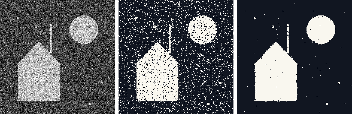
The middle panel shows the problem. Noise pushes many dark pixels above 0.5, and many bright pixels below it. In this test image, 3,881 of 36,864 pixels (about 11%) end up on the wrong side.

To fix this, a pixel must look at its neighbors. That is exactly what the boundary-length term does. But boundary length is awkward to work with. It belongs to the whole shape, not to any one pixel. If you flip one pixel, the boundary changes in a complicated way.

Earlier methods follow the curve directly, or they solve a large optimization problem. They work, but they are complex to build and can be slow.

The key idea

The trick is to measure boundary length with a blur.

Describe the inside group as a mask $u$: 1 for inside pixels, 0 for outside pixels. Now blur the mask with a Gaussian blur, the same blur that photo editors use.

Far from the boundary, nothing changes. A pixel deep inside sees only 1s around it, so it stays 1. Near the boundary, the blur leaks across. Inside pixels drop a bit below 1, and outside pixels rise a bit above 0.

The total amount of leak is proportional to the length of the boundary. A long, wiggly boundary leaks a lot. A short, smooth one leaks little. So "boundary length" turns into "how much the blurred mask leaks", and a blur is easy to compute.

With this trick, the method runs in rounds. Each round has four steps:

1. Compute the average brightness inside, $c_{\text{in}}$, and outside, $c_{\text{out}}$.
2. Blur the mask.
3. Give every pixel two scores, one for each side.
4. Move every pixel to the side with the lower score.

The two scores are:

The first part of each score asks: does my brightness match this side? The second part asks: do my neighbors belong to this side? The number $\kappa = 2\lambda\sqrt{\pi}/\sqrt{\delta t}$ sets how much the neighbors count.

So every pixel votes, using its own color and the opinion of its neighborhood. A lonely bright speck in a dark area has almost no inside neighbors. Its blurred mask value is close to 0, so its inside score is high, and it moves outside.

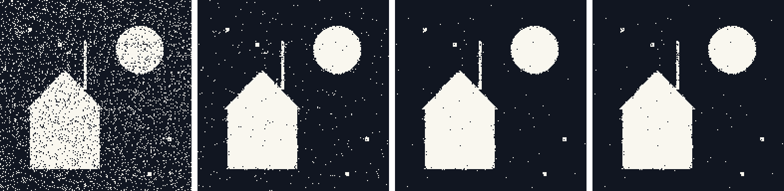
On the test image, round 1 cuts the wrong pixels from 3,881 to 426. Round 2 brings them to 187. After 7 rounds, no pixel switches sides any more, and the method stops.

Two facts make this method good, not just simple.

It always settles. The paper proves that the energy never goes up from one round to the next, for any blur width. So the method cannot cycle forever. In the paper's tests, it stopped after 7 to 20 rounds.

It is fast. The only expensive step is the blur. A fast Fourier transform does it in about $N \log N$ steps for $N$ pixels. For a four-region test, the round count stayed at 7 or 8 from 128×128 up to 512×512 pixels. The largest case took 0.67 seconds in MATLAB on a laptop.

The same idea works for more than two regions. Each pixel gets one score per region and joins the region with the lowest score. It also works for color images: the brightness difference becomes a color difference.

Choosing the boundary price

The price $\lambda$ decides what counts as noise and what counts as detail.

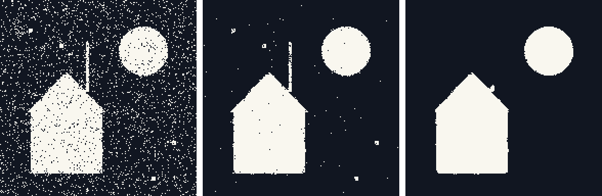
With a low price, short boundaries are cheap, so noise survives as specks. With a medium price, the noise goes, but the thin antenna and the small dots stay. With a high price, the antenna and the dots go too, because their boundary costs more than they save. There is no single right value. It depends on how small the smallest real feature is.

A link to today's AI

Look at one round again. It has two steps: a blur, then a choice made pixel by pixel.

The blur is a convolution, a linear operation that mixes each pixel with its neighbors. The choice is a simple nonlinear step: each pixel keeps the lower of two scores. A layer in a convolutional neural network has the same shape. It applies a convolution, then a pixel-by-pixel nonlinearity such as ReLU, which keeps positive values and sets negative ones to zero.

So seven rounds of this method look a lot like a seven-layer network. The difference is where the numbers come from. Here, math fixes every number: the blur is a Gaussian, and λ sets the weight. In a neural network, training on data picks the numbers. Researchers use this link on purpose. They turn an iterative method into a network and train its numbers. This is called algorithm unrolling.

The diffusion models that generate images today use the same family of ideas, in a different way. During training, they add noise to images, step by step, and learn to undo each step. Adding noise spreads the collection of all images the way heat spreads, by the same heat equation as our blur. Our method spreads one mask. A diffusion model spreads a whole probability distribution, and a trained network runs it backward. That network is itself a deep stack of linear layers and nonlinear steps.

Some researchers make the link even closer and use blur in place of noise. Examples are inverse heat dissipation and cold diffusion. The blur-then-decide idea from 1990s mathematics is still at work, now with learned numbers.

Try it yourself

This demo runs the same method in your browser. Press One round a few times and watch the specks disappear. Then change λ and run it again.

Behind the scenes

I wrote this paper with Dong Wang, Haohan Li and Xiaoping Wang at the Hong Kong University of Science and Technology. We posted it on arXiv in August 2016, and it appeared in the Journal of Computational Physics in 2017.

The idea of "blur, then threshold" is older than our paper. Merriman, Bence and Osher used it in the early 1990s to move curves by their curvature. Esedoğlu and Otto later showed how to use the blur to measure boundary length between many regions. Our paper brought that idea to image segmentation with the Chan–Vese score.

Go further

• The paper on arXiv, free to read: An efficient iterative thresholding method for image segmentation.
• The journal version: Journal of Computational Physics, 2017.
• MATLAB code for the method: threshseg.
• The classic blur-and-threshold scheme in C++: MBOX.
• The code for the figures in this post: make_figures.py.